Benchmarks
The results can be found here: benchmark-task-results
Benchmark Metrics
The basic metric for comparison is Time to Accuracy, i.e. training time of the system until a specified target accuracy is reached (where accuracy will be test and/or training accuracy).
The variable dimensions are:
Algorithm - limited number of prescribed standard algorithms, according to strict reference implementations provided
Hardware - GPU(s) - CPU(s) - Memory
Scalability - Number of workers
Network - Impact of bandwidth and latency
Benchmark Task Descriptions
We here provide precise descriptions of the official benchmark tasks. The task are selected to be representative of relevant machine learning workloads in both industry and in the academic community. The main goal here is a fair, reproducible and precise comparison of most state-of-the-art algorithms, frameworks, and hardware.
For each task, we provide a reference implementation, as well as results for different systems.
Task 0: Communication Backend Raw Performance
This task consists of benchmarking the communication backends for different frameworks and operations.
0.a All-reduce
In this task, tensors of increasing size in np.logspace(0, 8, num=80) are sent between workers, 100 times for each tensor size.
This allows for measuring and comparing the communication times for each backend for an all-reduce operation.
Task 1: Image Classification
1a. Resnet-20, CIFAR-10
Image classification is one of the most important problems in computer vision and a classic example of supervised machine learning.
- Model
We benchmark two model architectures of Deep Residual Networks (ResNets) based on prior work by He et al. The first model (m1) is based on the ResNets defined in [HZRS15]. The second version (m2) is based on the ResNets defined in [HZRS16]. For this benchmark implementation, we use 20 layers ResNet called ResNet-20 using the first version stated previously.
- Dataset
The CIFAR-10 dataset containing a set of images used to train machine learning and computer vision models. It contains 60,000 32x32 color images in 10 different classes, with 6000 images per class. The 10 different classes represent airplanes, cars, birds, cats, deer, dogs, frogs, horses, ships, and trucks.
The train / test split as provided in the dataset is used. The test dataset contains 10,000 images with exactly 1000 randomly-selected images per each class. The rest 50,000 images are training samples.
- Training Algorithm
We use standard synchronous SGD [DAM+16] as the optimizer (distributed mini-batch SGD with synchronous all-reduce communication before each mini-batch update).
number of machines
k = 1, 2, 4, 8, 16, 32minibatch size per worker
b = 128maximum epochs: 164
learning rate
learning rate \(\eta\) : 0.02
decay: We reduce the learning rate when a plateau in the validation loss is reached for 2 consecutive epochs
scaling and warmup: apply
linear scaling rulementioned in [GDollarG+17]. The learning rate is scaled from \(\eta\) to \(\eta \times k\) within the first \(log_{2}(num\_workers)\).
optimizer:
CentralizedSGD(momentum=0.9, nesterov=True, weight_decay=1e-4, dampening=0, by_layer=False)loss :
CrossEntropyLoss
Besides, in each round workers access disjoint set of datapoints.
Implementation details:
- Data Preprocessing
We followed the same approach described in [HZRS15].
- Selection of Framework & Systems
We aim to provide the same algorithm in multiple frameworks, primarily focusing on PyTorch and Tensorflow. For the systems, kubernetes allows easy transferability of our code. While initial results reported are from google kubernetes engine, AWS will be supported very soon.
- Environments for Scaling Task
We use a single process per node environment, with one GPU per process (i.e. one GPU per node). The bandwidth between two nodes is around 7.5Gbit/s.
MPI,GLOOorNCCLare used for communication.
1b. Resnet-?, ImageNet
TODO
Task 2: Linear Learning
2.a Logistic Regression, Epsilon 2008
- Model
We benchmark Logistic Regression with L2 regularization.
- Training Algorithm
We use standard synchronous SGD [DAM+16] as the optimizer (that is distributed mini-batch SGD with synchronous all-reduce communication before each mini-batch).
number of machines
k = 1, 2, 4, 8, 16minibatch size per worker
b = 128maximum epochs: 164
learning rate
learning rate \(\eta\) : 4
decay: We reduce the learning rate when a plateau in the validation loss is reached for 2 consecutive epochs
scaling: The learning rate is scaled from \(\eta\) to \(\eta \times k\) for \(k\) workers
optimizer:
CentralizedSGD(momentum=0, nesterov=False, weight_decay=0, dampening=0, by_layer=False)loss:
BCELossRegularized(Binary Cross-Entropy Loss with regularization)regularization parameters: \(L1=0, L2 = 0.0000025\)
Implementation details:
- Data Preprocessing
Dataset is pre-processed prior to training, and stored on [here](https://storage.googleapis.com/mlbench-datasets/libsvm). The pre-processing script can be found under mlbench_core/dataset/util/pytorch/libsvm.py, and generates .lmdb files from the original dataset. One can easily generate the used dataset by running:
$ python mlbench_core/dataset/util/pytorch/libsvm.py epsilon [test | train] [dest_dir]
- Selection of Framework & Systems
We aim to provide the same algorithm in multiple frameworks, primarily focusing on PyTorch and Tensorflow. For the systems, kubernetes allows easy transferability of our code. While initial results reported are from google kubernetes engine, AWS will be supported very soon.
- Environments for Scaling Task
We use a single process per node environment, with no GPU acceleration. The bandwidth between two nodes is around 7.5Gbit/s.
MPIorGLOOare used for communication.
Task 3: Language Modelling
3a. LSTM, Wikitext2
- Model
We benchmark the AWD-LSTM model.
- Dataset
The Wikitext2 dataset is used. contains text for language modelling. The train set contains 2088628 tokens, and the validation set 217646 tokens. The vocabulary is made up of 33278 words.
- Training Algorithm
We use standard synchronous SGD as the optimizer (that is distributed mini-batch SGD with synchronous all-reduce communication before each mini-batch).
number of machines
k = 1, 2, 4, 8, 16, 32minibatch size per worker
b = 80sentencesbackpropagation through time:
bptt_len = 70Sequence length: Sampled at random for each batch using the following rule
X ~ Bernouilli(0.05), seq_len = max(min_seq_len, Normal(bptt_len / (1 + X), 5))Validation sequence length: 10
maximum epochs: 750
optimization
learning rate per batch \(\eta = 30 \times \frac{seq\_len}{bptt\_len}\)
weight decay: \(1.2e-6\)
scaling: We use linear warm-up to scale the learning rate \(\eta\) to \(\eta \times \sqrt{num\_workers}\)
warm-up period: We use a warm-up period of \(num\_workers * 3\) epochs
gradient clipping: Gradient norm is clipped at 0.25
- scheduling:
If Perplexity stops improving for 5 epochs, optimizer is switched to Averaged SGD
- loss:
CrossEntropyLoss Activation regularization \(\alpha = 2\)
Temporal Activation reg. \(\beta = 1\)
- loss:
Implementation details:
- Selection of Framework & Systems
We aim to provide the same algorithm in multiple frameworks, primarily focusing on PyTorch and Tensorflow. For the systems, kubernetes allows easy transferability of our code.
- Environments for Scaling Task
We use a single process per node environment, with no GPU acceleration. The bandwidth between two nodes is around 7.5Gbit/s.
MPI,GLOOor NCCL are used for communication.
Task 4: Machine Translation
4.a LSTM, WMT16 EN-DE
- Model
We benchmark the GNMT Machine Translation Model [WSC+16], which follows the sequence-to-sequence learning framework, and uses stacked residual LSTM connections in the encoder and decoder modules. The residual connections allow for deeper stacked LSTM layers, as without residuals, the stack typically suffer from vanishing/exploding gradients when too many layers are used.
- Dataset
The WMT-16 dataset containing a set of translated sentences from multiple languages. We exclusively use English-German translation from this dataset.
The model is trained on sentences of maximum length 75 tokens, and tested on sentences of max length 150 tokens.
- Training Algorithm
We use Synchronous distributed Adam as the optimizer, which is similar to [DAM+16], but uses Adam’s update rule: Before each weight update, gradients on all workers are summed using an
all_reduceoperation; that way, all workers share their gradients and obtain the same weight update.Also, this training algorithm uses mixed precision training (explained below).
number of machines
k = 1, 2, 4, 8, 16, 32global minibatch size
b = 2048sentences 1maximum epochs: 8
learning rate (Figure 1. left plot)
initial_learning_rate = 0.0base_learning_rate = 2.0e-3decay: We decay by \(0.5\) after having gone through 40% of total training, and then for every 5% for maximum 4 times
scaling and warmup: We use 200 warmup steps, where the learning rate is exponentially increased from
initial_learning_ratetobase_learning_rate
optimizer:
Adam(betas=(0.9, 0.999), eps=1e-8, weight_decay=0, amsgrad=False)loss:
LabelSmoothingLoss(Negative Log-Likelihood with smoothing)gradient clipping: max norm of 5.0
Loss Scaling
initial_scale = 2**10scale_factor = 2(downscale and upscale)max_scale = 2**13scale_window = 128(steps after upscale if no overflow/underflow)
Implementation details:
- Data Preprocessing
The data needs to be downloaded and pre-processed and tokenized using the pre-processing script mlbench_core/dataset/nlp/pytorch/wmt16/preprocess/preprocess.py before training. The pre-processed data is available on our S3
- Mixed Precision Training
In order to have faster backward and forward passes, our model’s weights and gradients are cast into
float16prior to training.float32weights are still kept in memory and used by the optimizer to update weights. We use our ownFP16Optimizer. Sincefloat16has lower precision thanfloat32, it is necessary to have a loss scaler:Start with
loss_scale = initial_scaleBefore each backward pass, inflate the loss by
loss_scale(infloat16) to avoid under-flowsBefore weight update, deflate gradients by
loss_scale(infloat32) to keep precisionClip gradient norm to be
grad_clipCheck if gradient norm is
nanorinf(infloat16). If True,loss_scale = loss_scale / scale_factor. If False, update weights.If after
scale_windowupdates, no overflow/underflow detected,loss_scale = loss_scale * scale_factor
- Selection of Framework & Systems
We currently only have this reference implementation in PyTorch. For the systems, kubernetes allows easy transferability of our code. While initial results reported are from Google Kubernetes engine, AWS will be supported very soon.
- Environments for Scaling Task
We use a single process per node environment, with one GPU per process (i.e. one GPU per node). The bandwidth between two nodes is around 7.5Gbit/s.
MPIorNCCLare used for communication.
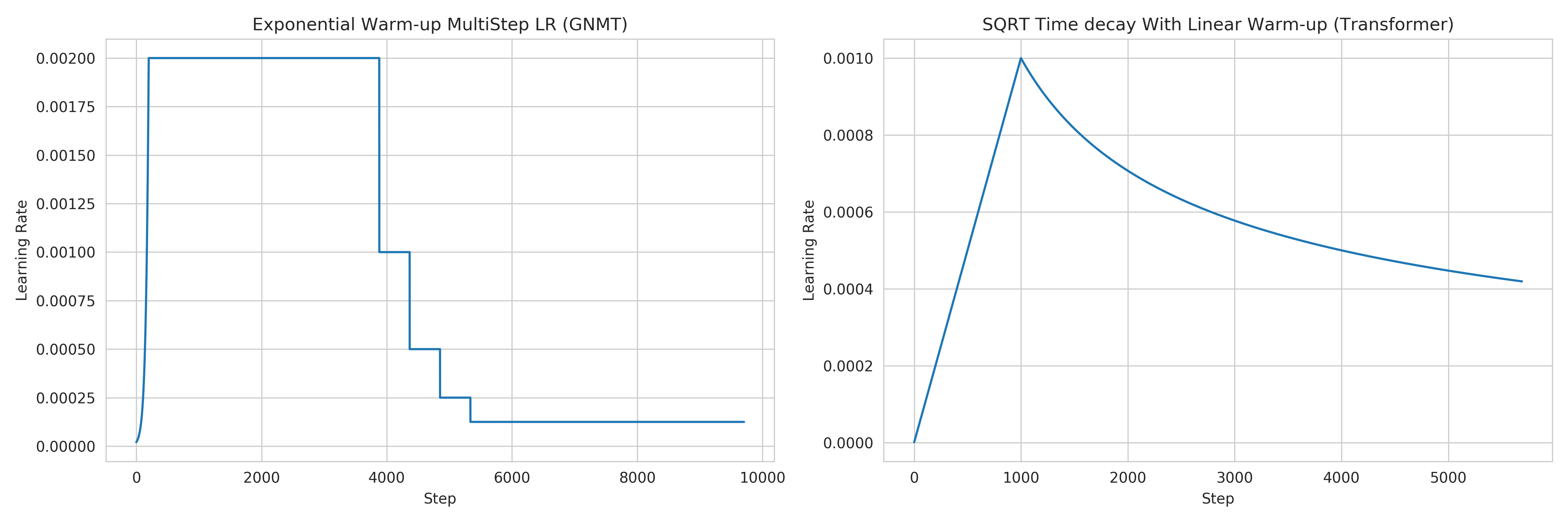
Figure 1: Learning rate scheduler for GNMT and Transformer
- 1(1,2)
Fitting batch in memory: In order to achieve the mentioned global batch size, one needs to fit a batch size of
bw = b / world_sizeon each worker. Depending on the used hardware, this cannot be achieved as it takes up too much memory. For that, we compute the gradients on multiple batches of smaller sizebsand aggregate them, before applying the weight update. The frequency at which we update is calledupdate_freq.This implies that the global batch size is
b = bs * world_size * update_freq. For the used hardware,max(bs) = bs_max = 128is the maximum value we can fit in memory. Thus, we haveupdate_freq = max(1, b / (bs_max * world_size))thusbs = b / (world_size * update_freq)
4.b Transformer, WMT17 EN-DE
- Model
We benchmark the Transformer Model, using attention mechanisms based on the paper “Attention Is All You need” [VSP+17] that. The implementation is based on a combination of NVIDIA’s implementation of fairseq ‘s transformer. Our implementation differs from MLPerf’s in one subtle way: the FusedLayerNorm layers are changed to native torch LayerNorm, as its performance has increased since. Also, instead of using FusedAdam, we use Adam. One part of the MultiheadAttention module needs a cuda extension, that makes training significantly faster than torch’s native MultiheadAttention
- Dataset
The WMT-17 dataset containing a set of translated sentences from multiple languages. We exclusively use English-German translation from this dataset.
The model is trained and tested on sentences of maximum length 80 tokens.
- Training Algorithm
We use Synchronous distributed Adam as the optimizer, which is similar to [DAM+16], but uses Adam’s update rule: Before each weight update, gradients on all workers are summed using an
all_reduceoperation and divided byworld_size * update_frequency; that way, all workers share their gradients and obtain the same weight update.Also, this training algorithm uses mixed precision training (explained below).
number of machines
k = 1, 2, 4, 8, 16, 32global minibatch size
b = 2**17tokens 2.maximum epochs: 10
learning rate (Figure 1. right plot)
initial_learning_rate = 0.0base_learning_rate = 1.976e-3decay: We decay by \(\sqrt{N}\) after warmup
scaling and warmup: We use 1000 warmup steps, where the learning rate is linearly increased from
initial_learning_ratetobase_learning_rate
optimizer:
Adam(betas=(0.9, 0.98), eps=1e-9, weight_decay=0, amsgrad=False)loss:
LabelSmoothingLoss(Negative Log-Likelihood with smoothing)Loss Scaling
initial_scale = 2**7scale_factor = 2(downscale and upscale)scale_window = 2000(steps after upscale if no overflow/underflow)
Implementation details:
- Data Preprocessing
The data needs to be downloaded and pre-processed and tokenized using the pre-processing script mlbench_core/dataset/nlp/pytorch/wmt17/preprocess/preprocess.py before training. The pre-processed data is available on our S3 storage
- Mixed Precision Training
In order to have faster backward and forward passes, our model’s weights and gradients are cast into
float16prior to training.float32weights are still kept in memory and used by the optimizer to update weights. We use our own FP16Optimizer. Sincefloat16has lower precision thanfloat32, it is necessary to have a loss scaler:Start with
loss_scale = initial_scaleBefore each backward pass, inflate the loss by
loss_scaling(infloat16) to avoid under-flowsBefore weight update, deflate gradients by
loss_scaling * full_batch_size / (world_size * update_freq)(infloat32) to keep precision, wherefull_batch_sizeis the batch size over all workers (sum of number of tokens on this batch for each worker).Check if gradient norm is
nanorinf(infloat16). If True,loss_scale = loss_scale / scale_factor. If False, update weights.If after
scale_windowupdates, no overflow/underflow detected,loss_scale = loss_scale * scale_factor
- Selection of Framework & Systems
We currently only have this reference implementation in PyTorch. For the systems, kubernetes allows easy transferability of our code. While initial results reported are from google kubernetes engine, AWS will be supported very soon.
- Environments for Scaling Task
We use a single process per node environment, with one GPU per process (i.e. one GPU per node). The bandwidth between two nodes is around 7.5Gbit/s.
MPIorNCCLare used for communication.
- 2
Fitting batch in memory: We apply the same technique as in 1. For the used hardware, we have
max(bs) = bs_max = 8192andupdate_freq = max(1, b / (bs_max * world_size))to getbs = b / (world_size * update_freq)
Benchmark Results
Here we present the results for scaling tasks. All results were generated on the Google Cloud Kubernetes Engine.
Task 0: Communication Backend
0.a PyTorch All-reduce
- Frameworks
PyTorch 1.5.0
- Communication Backends:
MPI (OpenMPI), GLOO and NCCL
- System Hardware
machine type: n1-standard-4 instances on GCP with 15GB memory and 4 virtual CPUs.
available CPUs: 3 CPUs available for pod (1 for Kubernetes management)
GPU: NVIDIA® Tesla® T4 (16GB GDDR6, Turing arch)
- Pricing
n1-standard-4: $0.2092/hour (regular), $0.0440/hour (preemptible)
NVIDIA® Tesla® T4: $0.35/hour (regular), $0.11/hour (preemptible)
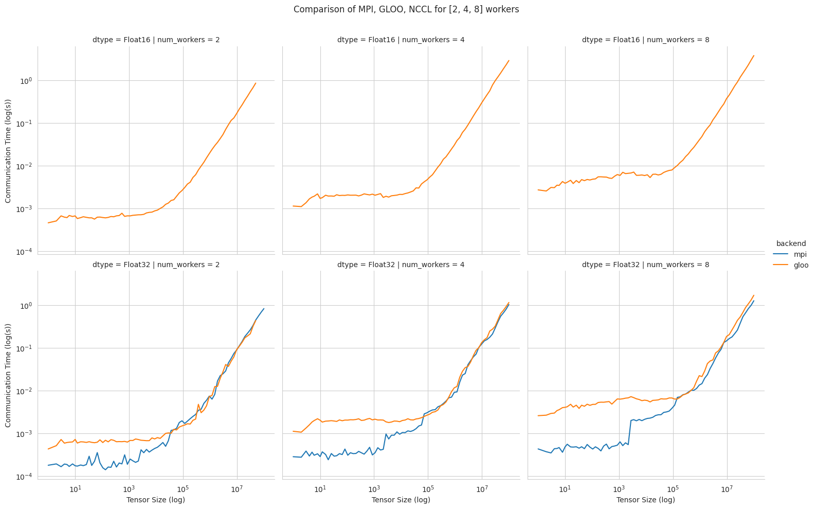
Communication for 2 to 8 workers (CPU tensors)
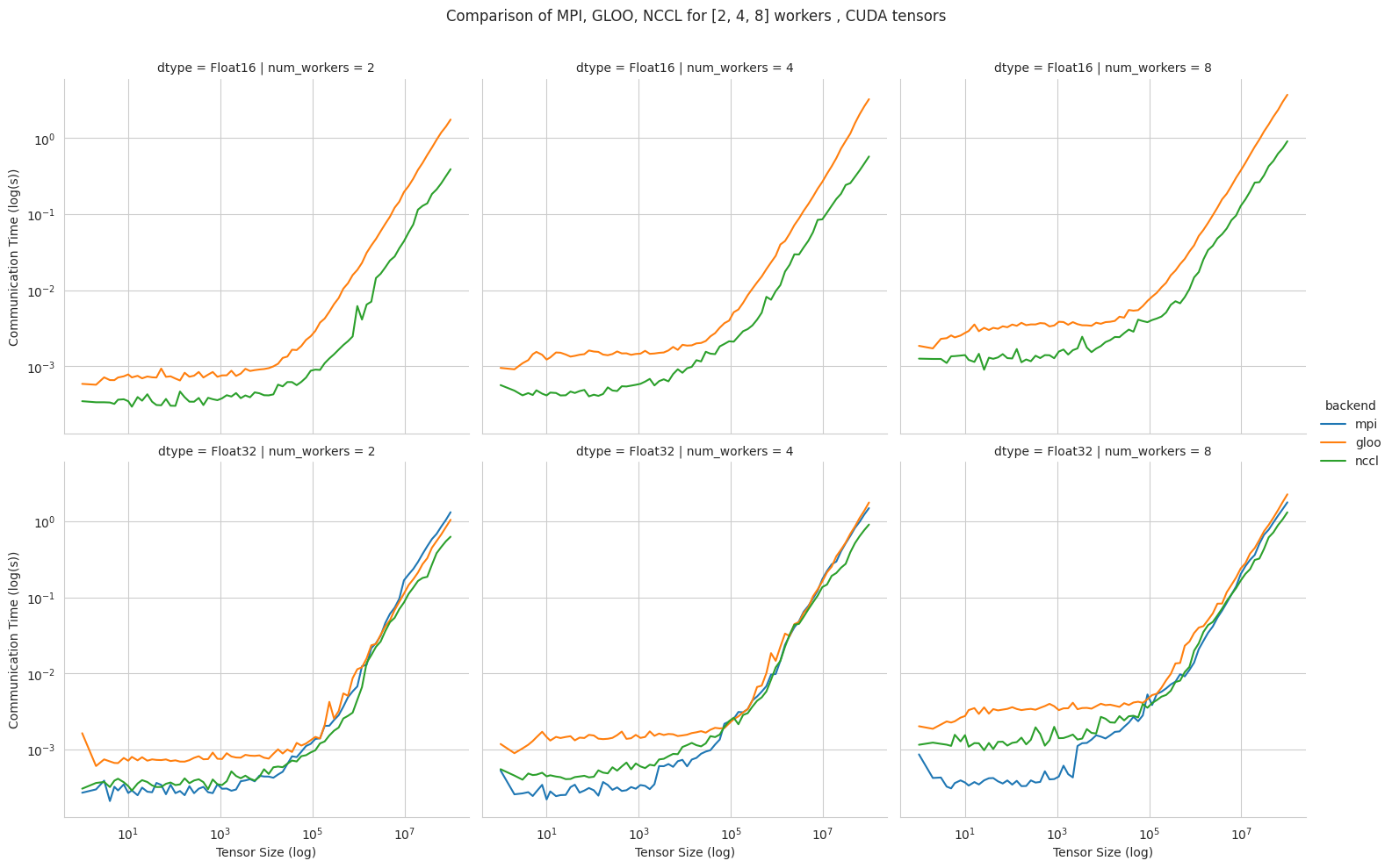
Communication for 2 to 8 workers (GPU tensors)
The first figure shows the communication times between 2, 4, and 8 workers for
float32andfloat16CPU tensors, for GLOO and MPI backends.The second figure shows the communication times between 2, 4, and 8 workers for
float32andfloat16GPU tensors, for GLOO, MPI and NCCL backends.MPI and GLOO both support CPU tensor communication, while NCCL only supports GPU tensors.
NCCL and GLOO both support
float16communication, while MPI only supportsfloat32.This graph allows for a quantitative comparison of the different backends, and to study their advantages/disadvantages.
We can see that MPI behaves better than GLOO for small
float32CPU tensors, with similar performance they get larger.MPI seems to be less affected by increased cluster sizes.
MPI and NCCL have comparable performance for 2 workers (for small tensors), but NCCL gets slower as cluster size increases.
NCCL always has better performance for very large tensors, and supports
float16, while MPI doesn’t.GLOO has poor performance compared to others, but has the main advantage to be the only backend supporting
float16training on CPU.
Task 1: Image Classification
1a. Resnet-20, CIFAR-10
- Frameworks
PyTorch 1.5.0
Tensorflow
- Communication Backends:
MPI (OpenMPI), GLOO and NCCL
- System Hardware
machine type: n1-standard-4 instances on GCP with 15GB memory and 4 virtual CPUs.
available CPUs: 3 CPUs available for pod (1 for Kubernetes management)
GPU: NVIDIA® Tesla® T4 (16GB GDDR6, Turing arch)
- Metric
Time to Accuracy of 80% on validation set.
- Pricing
n1-standard-4: $0.2092/hour (regular), $0.0440/hour (preemptible)
NVIDIA® Tesla® T4: $0.35/hour (regular), $0.11/hour (preemptible)
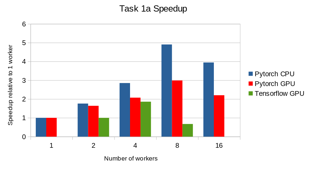
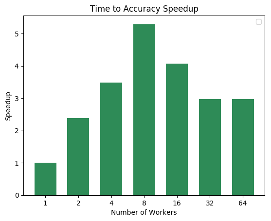
The next figure shows the speedup in training times to 80% accuracy relative to training on one node 3. The baseline time for 1 worker for the PyTorch CPU implementation is 5895 s, for the PyTorch GPU implementation 407 s and for the Tensorflow GPU implementation 1191 s.
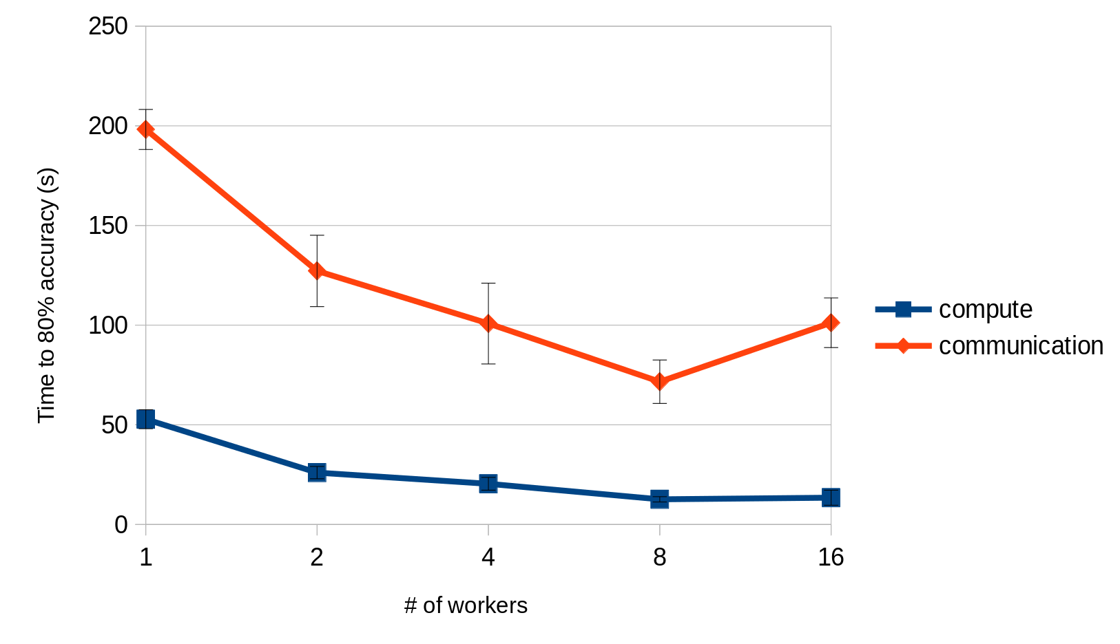
This figure shows the time spent in compute and communication for the PyTorch GPU implementation on 1, 2, 4, 8 and 16 workers.
The next figure compares the cost of experiment. Note that a regular n1-standard-4 instance costs $0.19 per hour and a preemptible one costs only $0.04. NVIDIA® Tesla® K80 GPUs (preemtpible) cost $0.135 per hour. All costs shown are for premtible instances.
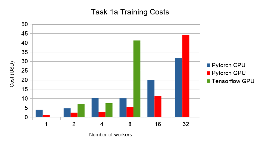
- 3
Training on CPU shows speedup with increasing number of nodes up to 32 nodes. For the Pytorch implementation on the GPU, speedups plateau at 4 nodes and decrease for 32 nodes. Tensorflow GPU numbers are only available up to 8 nodes, as more nodes lead to an Out-Of-Memory error on the GPU. This benchmark is still a work in progress and this issue will be fixed in a future release. Also since Tensorflow requires at least one parameter-server and a worker to run, it can’t be run on a single machine. As such, the results between PyTorch and Tensorflow are not directly comparable. Tuning the Tensorflow parameter-server in size when growing the number of total machines might require further tuning
1b. Resnet-?, ImageNet
TODO
Task 2: Linear Learning
2.a Logistic Regression, Epsilon 2008
- Frameworks
PyTorch 1.5.0
- Communication Backends:
MPI (OpenMPI), GLOO
- System Hardware
machine type: n1-standard-4 instances on GCP with 15GB memory and 4 virtual CPUs.
available CPUs: 3 CPUs available for pod (1 for Kubernetes management)
- Metric
Time to Accuracy of 80% on validation set.
- Pricing
n1-standard-4: $0.2092/hour (regular), $0.0440/hour (preemptible)
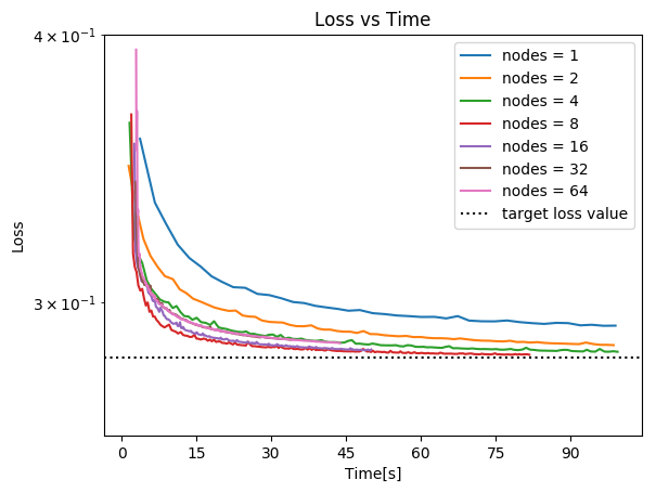
First figure shows the speedup of time to accuracy, for test accuracy of 89%, as the size of the cluster increases. Even though initially the speedup grows with the number of nodes added to the cluster, the benefit starts dropping for a cluster bigger than 16 nodes. This is mostly due to the issue of large-batch training. As the local batch-size of each worker is fixed, the global batch-size increases with the number of workers. Hence, while increasing batch size up to a point makes the training faster, beyond a certain point it will no longer reduce the number of training steps required, making it slower to reach the same accuracy.
Second figure illustrates how the loss value drops over time for various number of nodes. The black dotted line shows the target loss value, which is 0.2828 for this particular dataset.
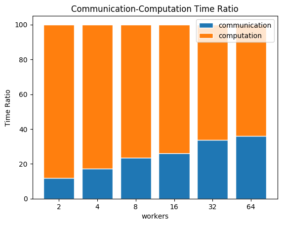
Last figure shows the average communication-computation time ratio for a node in the cluster. As we expected, the more workers we have, the more time is spent in communication.
Task 3: Language Modelling
3a. LSTM, Wikitext2
- Frameworks
PyTorch 1.7.0
- Communication Backends:
NCCL
- System Hardware
machine type: n1-standard-4 instances on GCP with 15GB memory and 4 virtual CPUs.
available CPUs: 3 CPUs available for pod (1 for Kubernetes management)
- Metric
Time to Perplexity of 70 on validation set
Task 4: Machine Translation
4.a LSTM, WMT16 EN-DE
- Frameworks
PyTorch 1.5.0
- Communication Backends:
NCCL
- System Hardware
machine type: n1-standard-4 instances on GCP with 15GB memory and 4 virtual CPUs.
available CPUs: 3 CPUs available for pod (1 for Kubernetes management)
GPU: NVIDIA® Tesla® T4 (16GB GDDR6, Turing arch)
- Metric
Time to BLEU-Score of 24.0 on test set.
- Pricing
n1-standard-4: $0.2092/hour (regular), $0.0440/hour (preemptible)
NVIDIA® Tesla® T4: $0.35/hour (regular), $0.11/hour (preemptible)
Training on 1 node ~10$
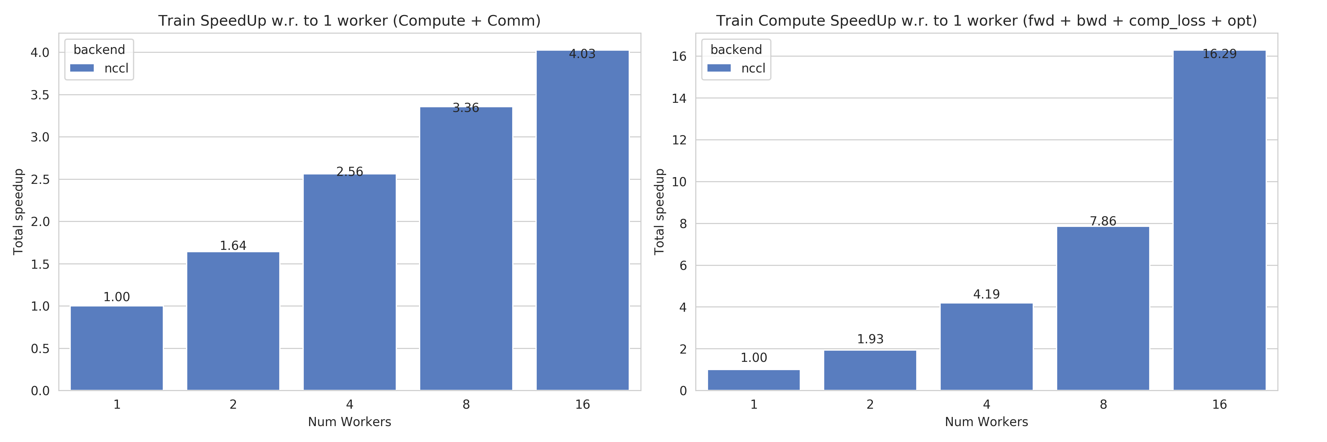
Speedups for Task 4a: with communication times (left), without (right)
This figures shows the absolute speedup (left), and the compute speedup (right). The compute speedup doesn’t account for communication times, and is only used as an indicator to see the maximum achievable speedup with lightspeed communication.
A few interesting points:
Overall speedups seem to follow logarithmic scaling for this configuration.
Scaling the number of compute nodes gives perfect linear scaling for this task
Using more powerful communication hardware (e.g.
NVLink®) will positively affect speedups.
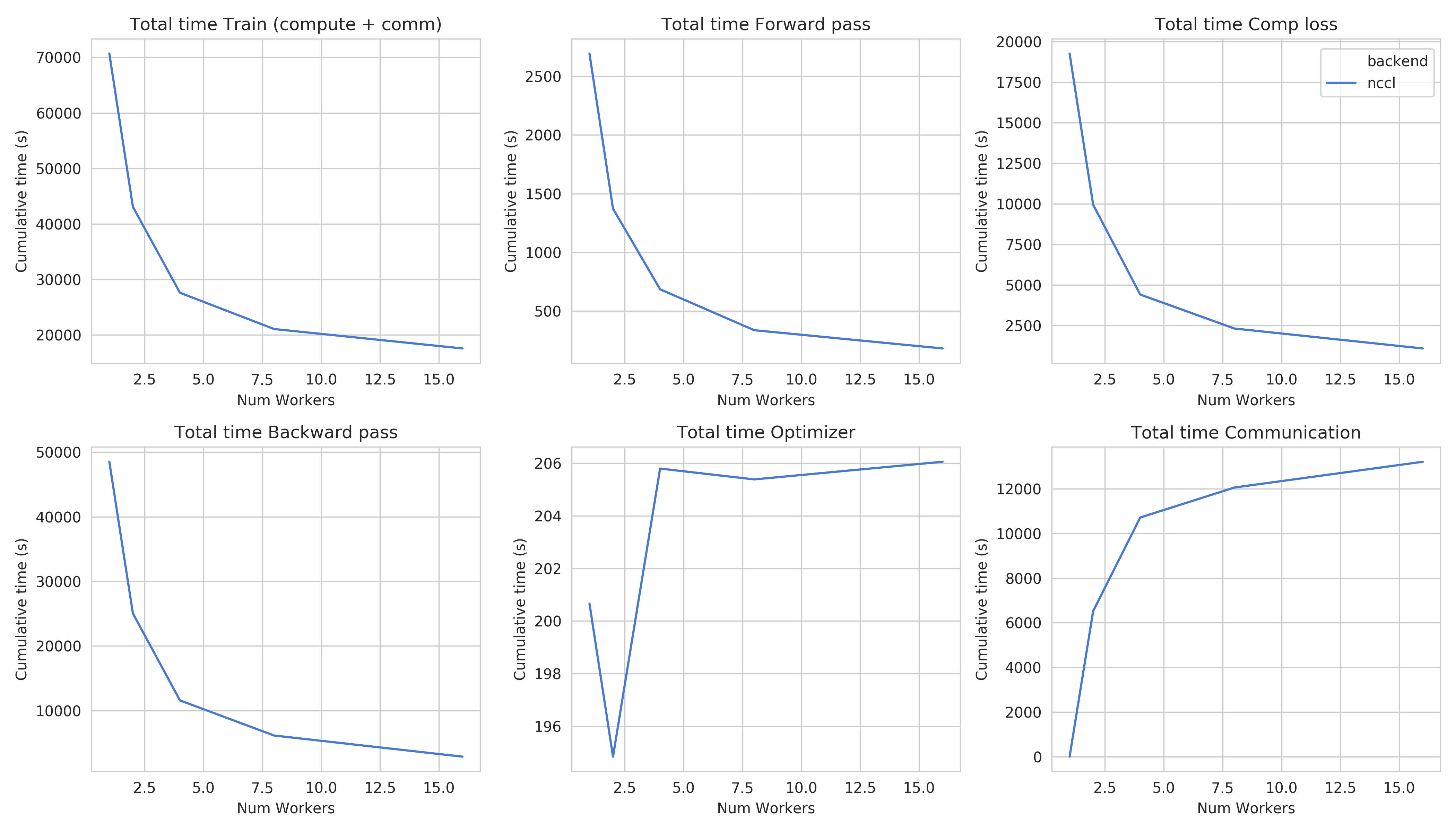
Step times for task 4a
This figure shows the total time spent in each step for all cluster sizes.
Total time and compute step times follow an exponential decay with the increase of number of nodes.
Time spent optimizing doesn’t seem to follow the same path, but increases are insignificant (~10 seconds), and are due to additional compute steps (averaging tensors, computations related to Mixed precision) when using distribution
Total communication time increases also logarithmically
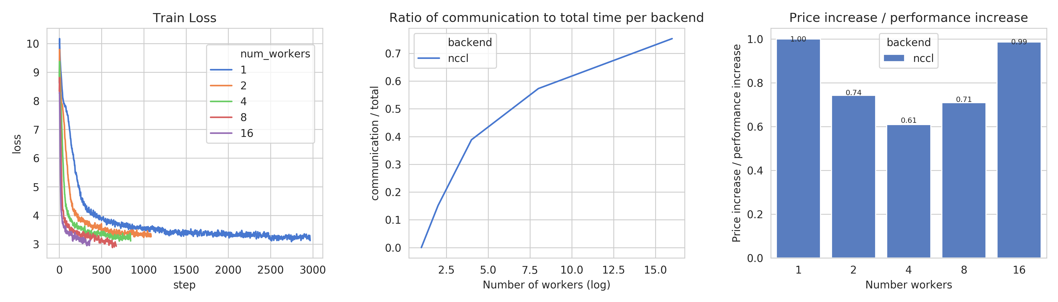
Train loss (right), Ratio of communication to total time, Price index for Task 4a
This figure shows, the train losses (right), Ratio of communication to total time, and a price index. The price index is computed as follows \(index = \frac{price\_increase}{performance\_increase}\)
The center graph is useful, as it depicts the limits of distribution for this model, using the described hardware. We can see that after 8 workers, communication takes up more than 50% of total time,
The right-most graph, shows the worthiness of distribution:
The price increase is less than the performance increase for 2, 4, and 8 workers. This suggests that distribution is worth the price increase
The 4 workers case seems to be the best price-performance trade-off.
Training on 4 workers costs ~18$, but is 2.56 times faster.
4.b Transformer, WMT17 EN-DE
- Frameworks
PyTorch 1.5.0
- Communication Backends:
NCCL
- System Hardware
machine type: n1-standard-4 instances on GCP with 15GB memory and 4 virtual CPUs.
available CPUs: 3 CPUs available for pod (1 for Kubernetes management)
GPU: NVIDIA® Tesla® T4 (16GB GDDR6, Turing arch)
- Metric
Time to BLEU-Score of 25.0 on test set.
- Pricing
n1-standard-4: $0.2092/hour (regular), $0.0440/hour (preemptible)
NVIDIA® Tesla® T4: $0.35/hour (regular), $0.11/hour (preemptible)
Training on 1 node ~5.5$
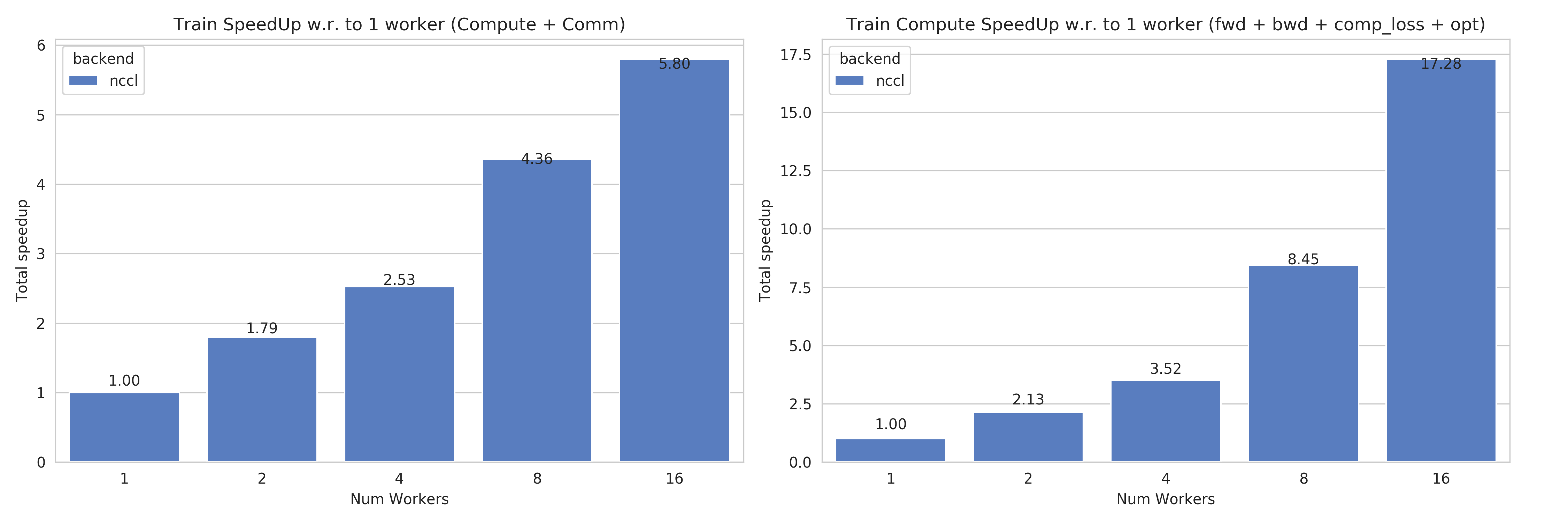
Speedups for Task 4b: with communication times (left), without (right)
This figures shows the absolute speedup (left), and the compute speedup (right). The compute speedup doesn’t account for communication times, and is only used as an indicator to see the maximum achievable speedup with lightspeed communication.
A few interesting points:
Overall speedups follow a similar path than Task 4a, with even better speedups when not considering communication.
Linear speedup of compute implies a nearly perfect scaling for this task.
Using more powerful communication hardware (e.g.
NVLink®) will also positively affect speedups.
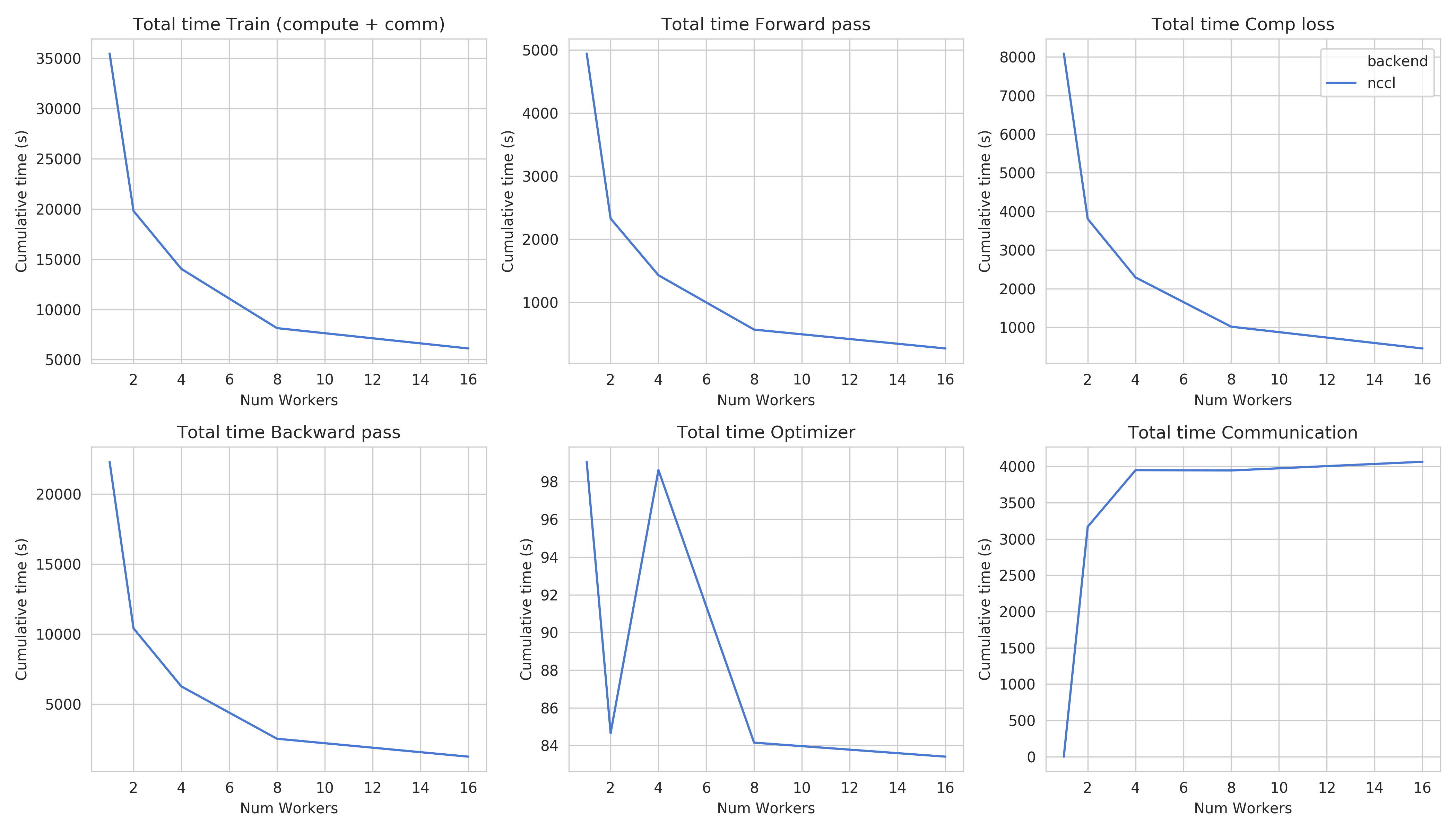
Step times for task 4b
This figure shows the total time spent in each step for all cluster sizes. We can observe very similar behaviour than Task 4a in all step times.
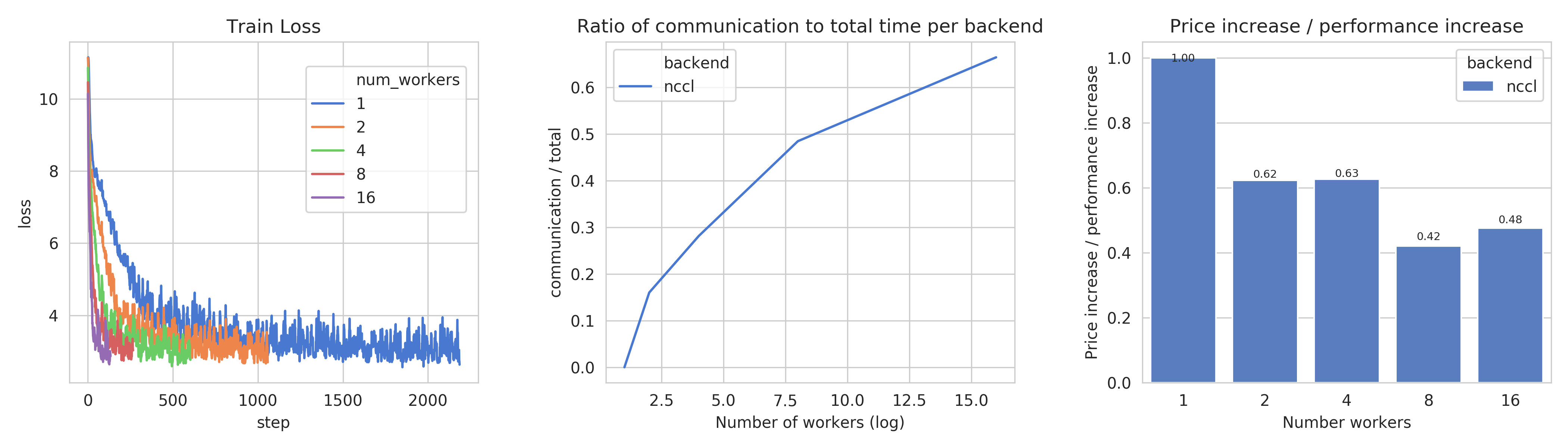
Train loss (right), Ratio of communication to total time, Price index for Task 4b
This figure shows, the train losses (right), Ratio of communication to total time, and a price index. Communication times ratio is lower than Task 4a for more workers, but still reaches over 50% for 8 workers.
The price index however, has a very different shape:
All price indices are below one.
This suggests that distributing this particular model on the mentioned hardware is always beneficial despite the price increase.
Training Transformer models seems to always benefit from distribution.
Training on most optimal configuration (8 workers) costs ~9.3$ and is 4.36 times faster.
Benchmark Task Implementations
For details on the available Benchmark implementations, please see Benchmark Implementations .
References
- DAM+16(1,2,3,4)
Dipankar Das, Sasikanth Avancha, Dheevatsa Mudigere, Karthikeyan Vaidyanathan, Srinivas Sridharan, Dhiraj D. Kalamkar, Bharat Kaul, and Pradeep Dubey. Distributed deep learning using synchronous stochastic gradient descent. CoRR, 2016. URL: http://arxiv.org/abs/1602.06709, arXiv:1602.06709.
- GDollarG+17
Priya Goyal, Piotr Dollár, Ross Girshick, Pieter Noordhuis, Lukasz Wesolowski, Aapo Kyrola, Andrew Tulloch, Yangqing Jia, and Kaiming He. Accurate, large minibatch sgd: training imagenet in 1 hour. arXiv preprint arXiv:1706.02677, 2017.
- HZRS15(1,2)
Kaiming He, Xiangyu Zhang, Shaoqing Ren, and Jian Sun. Deep residual learning for image recognition. CoRR, 2015. URL: http://arxiv.org/abs/1512.03385, arXiv:1512.03385.
- HZRS16
Kaiming He, Xiangyu Zhang, Shaoqing Ren, and Jian Sun. Identity mappings in deep residual networks. CoRR, 2016. URL: http://arxiv.org/abs/1603.05027, arXiv:1603.05027.
- VSP+17
Ashish Vaswani, Noam Shazeer, Niki Parmar, Jakob Uszkoreit, Llion Jones, Aidan N. Gomez, Lukasz Kaiser, and Illia Polosukhin. Attention is all you need. CoRR, 2017. URL: http://arxiv.org/abs/1706.03762, arXiv:1706.03762.
- WSC+16
Yonghui Wu, Mike Schuster, Zhifeng Chen, Quoc V. Le, Mohammad Norouzi, Wolfgang Macherey, Maxim Krikun, Yuan Cao, Qin Gao, Klaus Macherey, Jeff Klingner, Apurva Shah, Melvin Johnson, Xiaobing Liu, Lukasz Kaiser, Stephan Gouws, Yoshikiyo Kato, Taku Kudo, Hideto Kazawa, Keith Stevens, George Kurian, Nishant Patil, Wei Wang, Cliff Young, Jason Smith, Jason Riesa, Alex Rudnick, Oriol Vinyals, Greg Corrado, Macduff Hughes, and Jeffrey Dean. Google's neural machine translation system: bridging the gap between human and machine translation. CoRR, 2016. URL: http://arxiv.org/abs/1609.08144, arXiv:1609.08144.